Visualizing and handling flagged careless responses

Packages: dplyr, ggplot2, lubridate

There is still research ongoing on how to detect and to handle careless responses in the context of ESM studies. In addition, the threshold values that we use to detect careless responding are examples and don’t follow any recommendations. We strongly advice you to figure out which careless responding score(s) and threshold values are the most relevant for your study.

We began by detecting instances of negligent answering using the method(s) most applicable to your study at hand:

• Longstring
• Response time
• …

Identified cases of careless responding are marked with a ‘flag_cr’ value of 1. We now introduce diverse techniques that aid in understanding the prevalence of careless responding and whether it follows any particular patterns.

Describe

Initially, we can calculate either the count or the percentage of instances characterized by careless responding within the dataset. Additionaly, we can compute this percentage taking in account only the valid observations (valid==1).

sum(data$flag_cr == 1)

[1] 206

sum(data$flag_cr == 1) / nrow(data)

[1] 0.04904762

df_ = data[data$valid==1,]
sum(df_$flag_cr == 1) / nrow(df_)

[1] 0.04955872

The next plot offers a comprehensive perspective on the prevalence of careless responding throughout the study’s duration. Indeed, we can pinpoint instances of careless responding in relation to specific beep numbers and participant identifiers, providing an insightful overview.

data %>%
    ggplot(aes(x=obsno, y=factor(id), fill=factor(flag_cr))) +
        geom_tile(lwd = .5,
                  linetype = 1) +
  coord_fixed() +
  scale_fill_manual(values = c("grey","red"))

Additionnaly, we might also be interested in the variance of careless response occurrences, both within and between different contexts. One way is to represent the quantity and the distribution of the careless response over the participant. Over the next plots, two types of representations are useful:

• Absolute: maintains the original values, providing a clear view on the actual numbers of careless responding without any alteration.
• Relative: involves presenting values relative to the total quantity of observations. This consideration becomes pertinent especially when there are variations in the total number of observations across categories, yet the intention remains to examine disparities in proportions.

Note that to change representation, you only need to specify the position argument in the ‘geom_col()’ function (“stack” for absolute and “fill” for relative). Hence, we can represent the quantity and distribution over:

1. Participants
2. Study duration (observation number)
3. Specific period such as moments in a day (morning vs. afternoon vs. evening) or day type (weekend vs. weekday)

data %>% filter(valid==1) %>% 
    group_by(id, flag_cr) %>%
    summarise(n_flag_cr = n()) %>%
    ggplot(aes(y=n_flag_cr, x=factor(id), fill=factor(flag_cr))) +
        geom_col(position="stack") +
        coord_flip()

data %>% filter(valid==1) %>% 
    group_by(id, flag_cr) %>%
    summarise(n_flag_cr = n()) %>%
    ggplot(aes(y=n_flag_cr, x=factor(id), fill=factor(flag_cr))) +
        geom_col(position="fill") +
        coord_flip()

data %>% filter(valid==1) %>% 
    group_by(obsno, flag_cr) %>%
    summarise(n_flag_cr = n()) %>%
    ggplot(aes(y=n_flag_cr, x=obsno, fill=factor(flag_cr))) +
        geom_col(position="stack")

data %>% filter(valid==1) %>% 
    group_by(obsno, flag_cr) %>%
    summarise(n_flag_cr = n()) %>%
    ggplot(aes(y=n_flag_cr, x=obsno, fill=factor(flag_cr))) +
        geom_col(position="fill")

data %>% filter(valid==1) %>% 
    group_by(period, flag_cr) %>%
    summarise(n_flag_cr = n()) %>%
    ggplot(aes(y=n_flag_cr, x=period, fill=factor(flag_cr))) +
        geom_col(position="stack")

data %>% filter(valid==1) %>% 
    mutate(wday = ifelse(wday(sent) %in% c(1,7), "weekend", "weekday")) %>%
    group_by(wday, flag_cr) %>%
    summarise(n_flag_cr = n()) %>%
    ggplot(aes(y=n_flag_cr, x=wday, fill=factor(flag_cr))) +
        geom_col(position="fill")

Impact of careless reponding

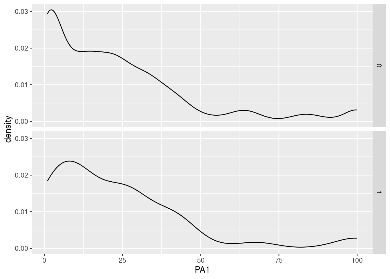
Because careless responding can bias collected data, it can have a significant impact on the quality of the collected data. In particular, careless responding can result in a skewed (e.g., over-consistent responses) or non-representative distribution (e.g., random response that increase variability). Hence, we can look at the distribution of a variable of interest separately for cases flagged for careless responding and normal cases:

data %>%
    ggplot(aes(x=PA1)) +
        geom_histogram() +
        facet_grid(flag_cr~., scales="free_y")

data %>%
    ggplot(aes(x=PA1)) +
        geom_density() +
        facet_grid(flag_cr~.)

Treating careless responding

The presence of careless responding has the potential to introduce bias and compromise the integrity of derived results and conclusions. This phenomenon adds unwanted noise and variance to the dataset, possibly obscuring genuine relationships between variables. Therefore, treating careless responding may improve the quality and reliability of the results and conclusions obtained from the data.

Various approaches exist for handling this issue, and the most suitable strategy should be tailored to match your specific study and analytical context. For instance, you could consider:

• Retaining the careless responses while accounting for them within the statistical model.
• Disregarding these responses during analysis while retaining the corresponding rows can be achieved by imputing missing values for the pertinent variables.

vars = c("PA1","PA2","PA3","NA1","NA2","NA3")
data[data$flag_cr==1, vars] = NA