Response time

Packages: dplyr, skimr

Warning

There is still research ongoing on how to detect and to handle careless responses in the context of ESM studies. In addition, the threshold values that we use to detect careless responding are examples and don’t follow any recommendations. We strongly advice you to figure out which careless responding score(s) and threshold values are the most relevant for your study.

Response times refer to the amount of time it takes for participants to provide a response to (time to fill) or open the survey (time to start). It can offer valuable information about participants’ engagement levels, and the effort they invest in responding to the survey items. In other words, it is thought to refer to careless responding with the idea that outliers or unexpected durations are worth investigating. As this topic deals with time to fill and time to start, you may find further relevant information in the Delay to start and to fill section.

First, we need to compute the response time (either time to fill or time to start) for each observation.

data = data %>% 
    mutate(time_int_start = start - sent, 
           time_int_fill = end - start) 

Plots

We propose to use a set of descriptive plots to investigate the overall but also the within and between difference in the response time (the Delay to start and to fill section contains further useful plots). In particular, and for both ‘time to start’ and ‘time to fill’ values, we propose to investigate:

• the distributions:

data %>% filter(valid==1) %>% 
    ggplot(aes(x=time_int_start)) +
        geom_histogram()

data %>% filter(valid==1) %>% 
    ggplot(aes(x=time_int_fill)) +
        geom_histogram()

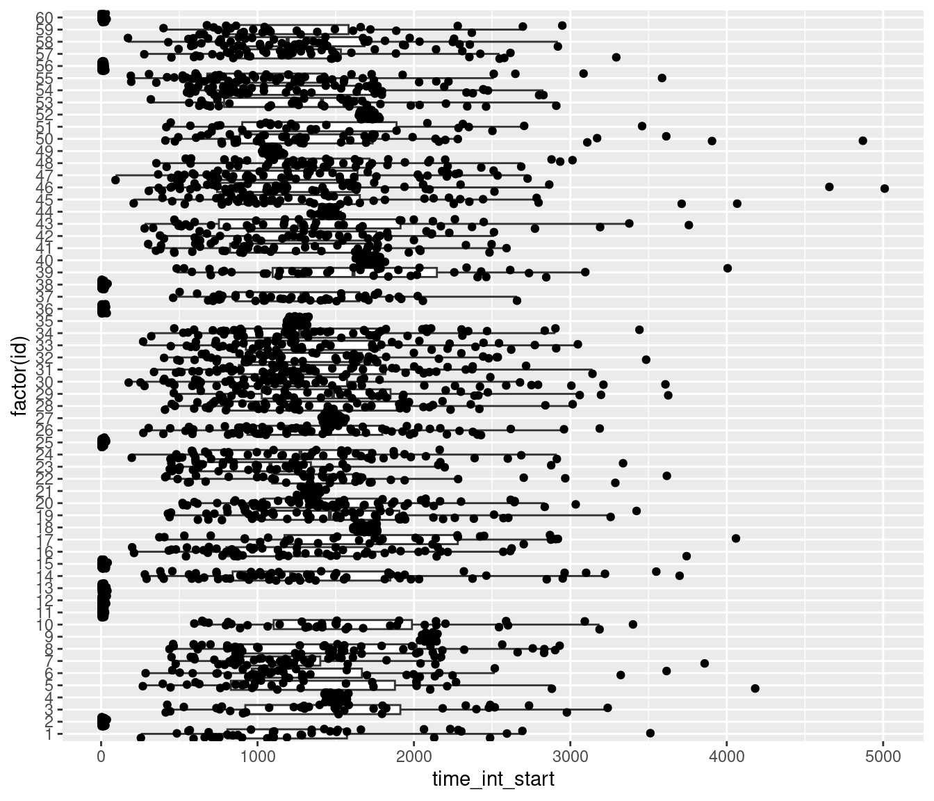
• the within and between variances:

data %>% filter(valid==1) %>% 
    ggplot(aes(y=time_int_start,x=factor(id))) +
        geom_boxplot(outlier.shape = NA) +
        geom_jitter() +
        coord_flip()

data %>% filter(valid==1) %>% 
    ggplot(aes(y=time_int_fill,x=factor(id))) +
        geom_boxplot(outlier.shape = NA) +
        geom_jitter() +
        coord_flip()

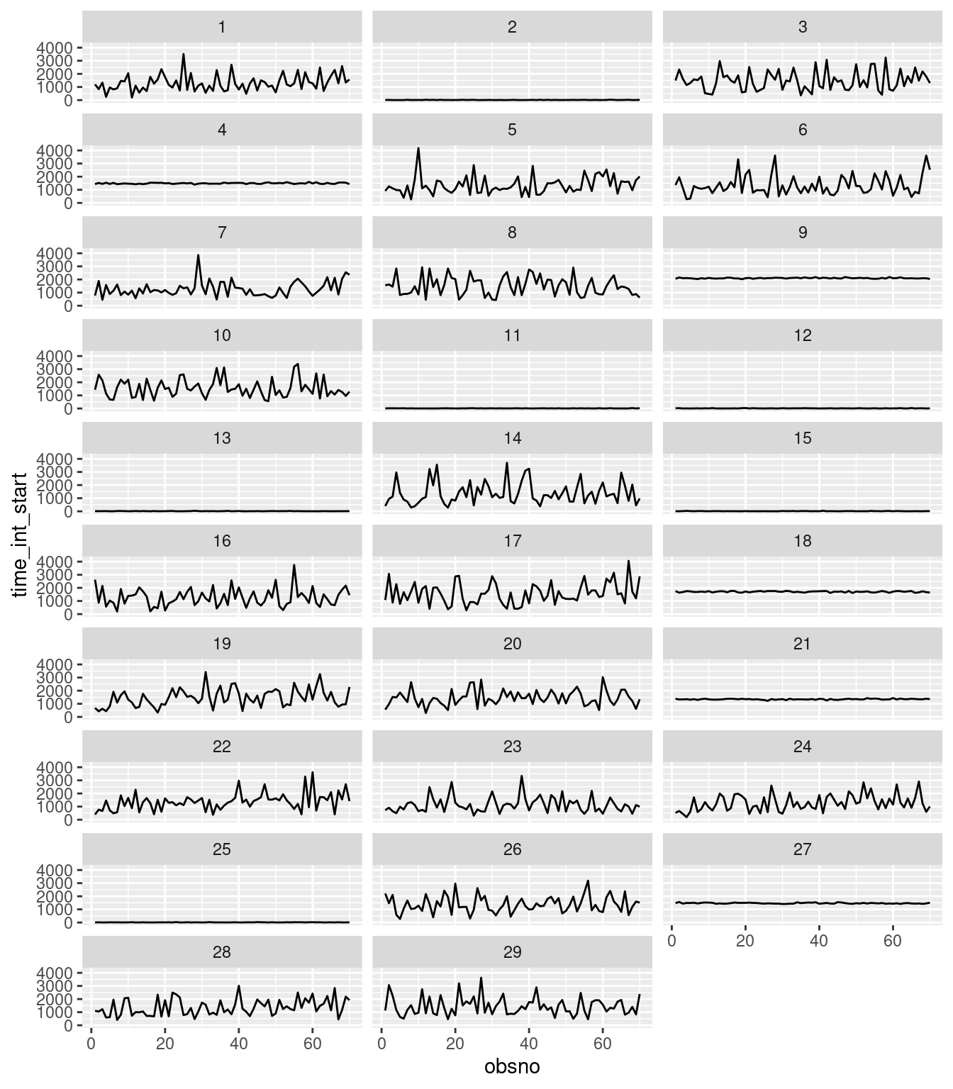
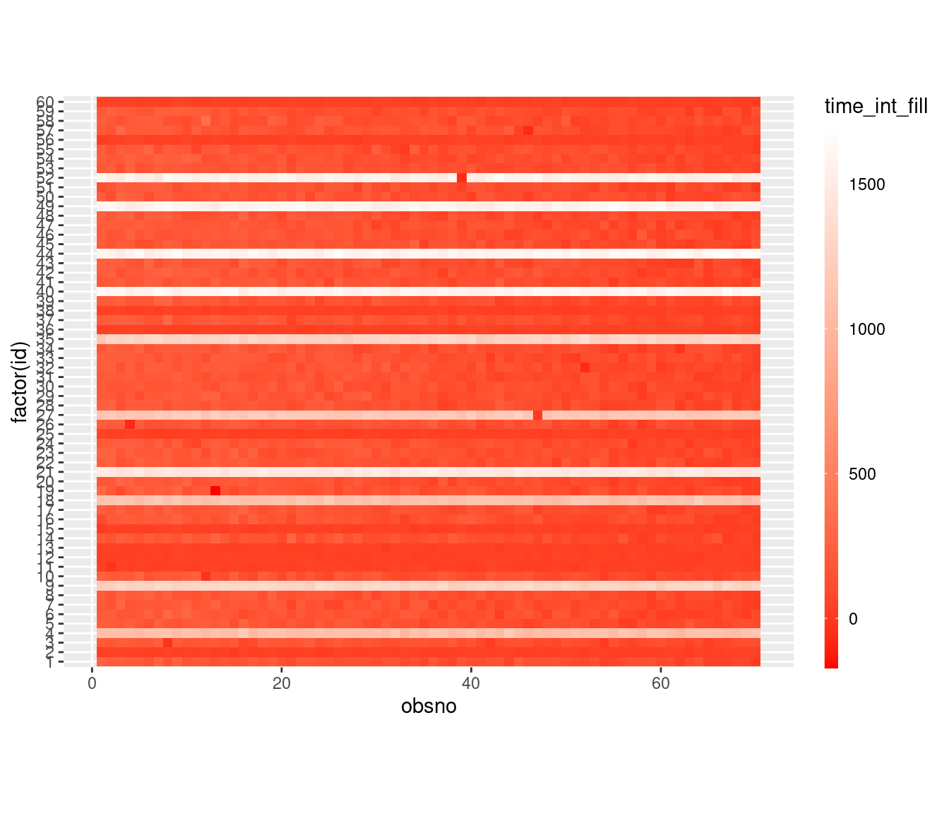
• the difference over the study duration within each participants using a heatmap or line plots (for a subset of participants):

data %>%
    mutate(time_int_start = as.numeric(time_int_start)) %>%
    ggplot(aes(x=obsno, y=factor(id), fill=time_int_start)) +
        geom_tile(lwd = .5, linetype = 1) +
        coord_fixed() +
        scale_fill_gradient(low = "red", high = "white") +
        guides(fill = guide_colourbar(barwidth = 0.5, barheight = 20))

data %>% 
    filter(id < 30) %>%
    ggplot(aes(x=obsno, y=time_int_start)) +
        geom_line() +
        facet_wrap(.~id, ncol=3)

data %>%
    mutate(time_int_fill = as.numeric(time_int_fill)) %>%
    ggplot(aes(x=obsno, y=factor(id), fill=time_int_fill)) +
        geom_tile(lwd = .5, linetype = 1) +
        coord_fixed() +
        scale_fill_gradient(low = "red", high = "white") +
        guides(fill = guide_colourbar(barwidth = 0.5, barheight = 20))

data %>% 
    filter(id < 30) %>%
    ggplot(aes(x=obsno, y=time_int_fill)) +
        geom_line() +
        facet_wrap(.~id, ncol=3)

Below 0

One challenge that can arise is encountering negative values for ‘time_to_start’ and ‘time_to_fill’ variables. These issues are often associated with the data collection application and server and may have been addressed during the second step of the ESM preprocessing framework. However, if you still encounter such values, they may require handling.

For instance, the following code calculates the count of ‘time_int_fill’ values that are less than zero:

sum(data$time_int_fill < 0)

[1] 10

Since there are 10 observations with values below zero, (following a thorough investigation,) we have chosen not to include these values in the subsequent analysis. Consequently, we eliminate the affected items using the following procedure:

nvars = c("PA1","PA2","PA3","NA1","NA2","NA3")

data[data$time_int_fill < 0, nvars] = NA

Flagging and handling cr obs

We propose two methods to decide on and flag the observations that are defined as careless responses. Both methods are using thresholds:

• Threshold 1: based on a number of standard deviations from the mean. Here we use 3 standard deviations.

time_int = data$time_int_start
thres_low = mean(time_int) - 3 * sd(time_int)
thres_high = mean(time_int) + 3 * sd(time_int)

• Threshold 2: absolute threshold.

thres_low = 0
thres_high = 1000 # in secs

In the following process, we apply the chosen threshold. The “flag_cr” variable will retain this information and will prove to useful in a later stage.

data$flag_cr = 0
data[data$time_int_fill > thres_low & data$time_int_fill < thres_high, "flag_cr"] = 1

Other descriptives can be found here: Visualizing and handling flagged careless responses