CR Longstring
There is still research ongoing on how to detect and to handle careless responses in the context of ESM studies. In addition, the threshold values that we use to detect careless responding are examples and don’t follow any recommendations. We strongly advice you to figure out which careless responding score(s) and threshold values are the most relevant for your study.
Longstring (Curran, 2016; Huang et al., 2012; Meade & Craig, 2012) is a technique used to detect over-consistent responses, indicating careless responding. This method implies the search for the longest string of identical responses for each observation (e.g., 1 1 1 1). In other words, it computes the number of times a particular response was selected in a row for each observation. There are different ways to compute such a longstring for each observation independently:
- count the maximal number of similar occurance in a row.
- compute an average of longest strings per page of survey.
- compute a weigthed score by averaging the length of the response.
For instance, we compute the longstring for the following response string from a Lickert scale item:
[1] 3 1 2 2 2 1 2 3 3In this example, the number ‘2’ is repeted 3 times in a row (the fourth time is apart from the rest). The maximal longstring score of this observation is then 3 (not ‘2’). Note that there is no consensus on a cut-off score that determine careless responses.
Reorder values
In ESM studies the items are answered multiple times by participants. A good practice to avoid habituation and contamination effects is to present the items in a random order. Hence, to be able to compute the longstring score, the original order of presentation (which was different per observation) must be known.
We have created a dataset in which the participant answers items in a random order for each presentaion. The first rows looks like:
head(data) %>% dplyr::select(PA1:NA3) PA1 PA2 PA3 NA1 NA2 NA3
1 52 78 15 67 47 75
2 75 66 15 71 93 64
3 57 86 21 73 97 44
4 43 38 75 1 71 13
5 63 93 44 58 38 98
6 62 98 20 55 5 70For our example, we stored the original order of the 6 items for each observation in another dataframe. Here are the first rows:
head(df_vars_order) X1 X2 X3 X4 X5 X6
1 NA1 PA2 NA2 PA1 NA3 PA3
2 PA1 NA2 PA2 NA1 NA3 PA3
3 PA2 NA1 NA3 NA2 PA3 PA1
4 NA1 NA3 PA1 PA3 PA2 NA2
5 NA2 PA2 PA1 NA3 PA3 NA1
6 PA3 NA1 NA2 NA3 PA1 PA2Based on this, we create a new dataframe ‘data_ordered’ that will store the values in the order of presentation, the one that is displayed in ‘df_vars_order’. During this process, we lose the ability to associate values with their respective variables. As a result, the dataset becomes valuable only for computing longstring scores for each observation.
# Extract variables names
var_names = c("PA1","PA2","PA3","NA1","NA2","NA3")

# Create empty dataframe that will store the correct order of the responses
data_ordered = as.data.frame(matrix(NA, nrow(data), length(var_names)))

# Takes the variable order of each row and fills the empty dataframe with the values in a correct order.
for (row in 1:nrow(df_vars_order)){
    order = unlist(df_vars_order[1,])
    data_ordered[row,] = data[row,order]
}
The output dataframe looks like:
head(data_ordered) V1 V2 V3 V4 V5 V6
1 67 78 47 52 75 15
2 71 66 93 75 64 15
3 73 86 97 57 44 21
4 1 38 71 43 13 75
5 58 93 38 63 98 44
6 55 98 5 62 70 20You may have to adapt the method in function of how the true order of presentation has been stored (e.g., in a character string, in a text file).
Longstring computation
careless package
The longstring function from the careless R package calculates the length of the longest string of identical responses for each participant. The longstring function also provides several options for handling missing data and can be customized to fit the needs of the user.
library(careless)We will compute longstring for answers from visual analogue scales in the ‘data’ dataframe. To do so, we first select the variables of interest (i.e., ‘PA1’ to ‘NA3’)
var_targeted = c("PA1","PA2","PA3","NA1","NA2","NA3")
df_subset = data[,var_targeted]
Then run the function on the subset of data. This function allows to compute:
- The maximal longstring number
data$longstring = careless::longstring(df_subset)- The average longstring (along with the maximal longstring) value with the avg argument
data[,c("longstring","longstring_avg")] = careless::longstring(df_subset, avg=TRUE)Here are the output values:
head(data[,c("id","obsno","longstring","longstring_avg")]) id obsno longstring longstring_avg
1 1 1 1 1
2 1 2 1 1
3 1 3 1 1
4 1 4 1 1
5 1 5 1 1
6 1 6 1 1As you can see, the longest string of equal values in the first lines is only 2. Of course, the probability of finding a longer string increases when the scale is smaller. For instance, on a Lickert scale with only 5 possible values, you are more likely to repeat values than on a visual analogue scale with 101 possible values.
esmtools package
The previous function indicates the maximal and average longstring scores but it does not mention for which value it was. To overcome this, we will use the ‘longstring()’ function from the esmtools. Here is the procedure:
- Select a subset of variables of interest
var_targeted = c("PA1","PA2","PA3","NA1","NA2","NA3")
df_ = data %>% dplyr::select(var_targeted)- Use the ‘longstring()’ function for each row. The function returns three outputs for each observation: value that has the maximal longstring, maximal longstring value, average longstring value.
library(esmtools)
# Compute longstring
mat_longstring = esmtools::longstring(df_)

# Merge longstring with the main dataframe and convert to numeric
data[,c("val_longstring","longstring","longstring_avg")] = mat_longstring
data = data %>% mutate(across(c(longstring, longstring_avg), as.numeric))
Here are the output values:
head(data[,c("id","obsno","val_longstring","longstring","longstring_avg")]) id obsno val_longstring longstring longstring_avg
1 1 1 multi 1 1
2 1 2 multi 1 1
3 1 3 multi 1 1
4 1 4 multi 1 1
5 1 5 multi 1 1
6 1 6 multi 1 1When the “val_longstring” designation is “multi,” it signifies that multiple values share the highest longstring value. For instance, if the maximum longstring value is 1, then multiple values will possess this top longstring value. In such cases, the “val_longstring” variable will indicate “multi” for that specific observation.
Descriptive analysis
Now that we have computed the longstring values, we can run descriptive statistics to investigate their occurence and if they follow specific patterns (e.g., participant high number of careless responses).
Occurence and distribution
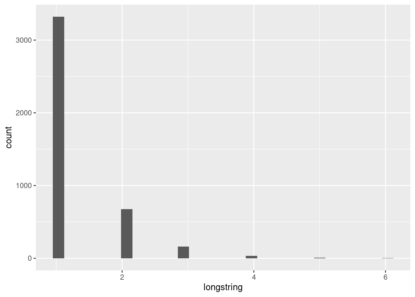
First, we can have a look at the distribution, or in other words, the occurence of the number of longstring values.
data %>%
    filter(!is.na(val_longstring)) %>%
    ggplot(aes(x=longstring)) +
        geom_bar()
We can investigate the within and between difference in the longstring values. For instance, we can also display the longstring values per participant. It would help investigate potential outliers within and between participants.
data %>%
    ggplot(aes(y=longstring, x=factor(id))) +
        geom_boxplot(outlier.shape = NA) +
        geom_jitter(size=.5) +
        coord_flip()
Additionnaly, we can investigate if the time has an effect on the longstring values. Hence, we can visualize:
- the number of occurence of longstring values per observation number (obsno).
data %>%
    group_by(obsno, longstring) %>%
    summarise(n_longstring = n()) %>%
    ggplot(aes(y=n_longstring, x=obsno, fill=longstring)) +
        geom_col()
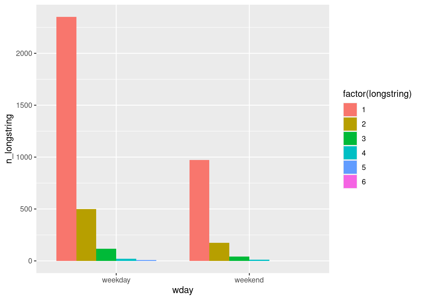
- the number of occurence of longstring values in the function of the week day vs. weekend day.
data %>%
    mutate(wday = ifelse(wday(sent) %in% c(1,7), "weekend", "weekday")) %>%
    group_by(wday, longstring) %>%
    summarise(n_longstring = n()) %>%
    ggplot(aes(y=n_longstring, x=wday, fill=factor(longstring))) +
        geom_col(position="dodge")
Which value is often the maximal longstring?
Because the longstring function from the esmtools pacakge gathers which values gives the maximal number longstring for each observation, we can plot this information as well. As with the previous values, we could also investigate the within and between participant variance for this score.
levels_ = c(as.character(1:100), "multi", NA)

data %>%
    group_by(val_longstring, longstring) %>%
    summarise(n_longstring = n()) %>%
    separate_rows(val_longstring, sep="_") %>%
    complete(val_longstring = levels_) %>%
    mutate(val_longstring = factor(val_longstring, levels=levels_)) %>%
    ggplot(aes(y=n_longstring, x=val_longstring, fill=factor(longstring))) +
        geom_col(position="stack") +
        scale_x_discrete(breaks = c(as.character(seq(0,100,10)), "multi", NA))
Flagging and handling cr obs
As detecting careless responses requires setting a threshold value, researchers must make subjective decisions about what to consider careless, which can impact the data quality and research findings. Therefore, it is important to carefully consider and justify the chosen threshold value when flagging observations as careless responses.
In the following process, we establish a arbitrary threshold of 4 and identify each observation where the maximum longstring value is greater than or equal to this threshold as indicative of careless responses. The “flag_cr” variable will retain this information.
threshold = 4

data$flag_cr = 0
data[data$longstring >= threshold & !is.na(data$longstring), "flag_cr"] = 1
For analyzing and handling flagged observations, you can take a look at the Visualizing and handling flagged careless responses section.


