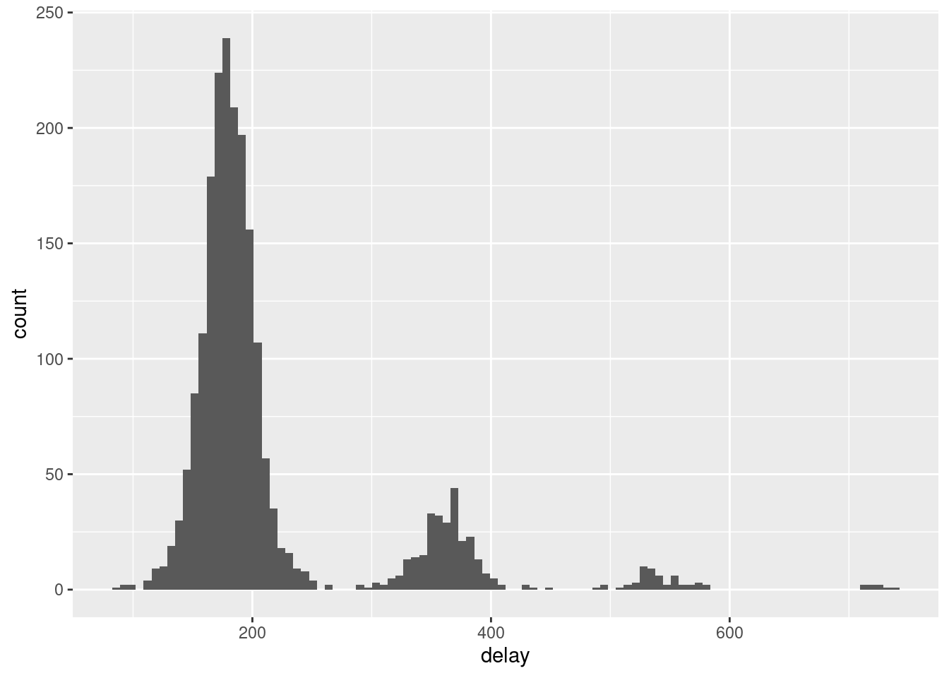
Delay between two consecutive and answered beeps

Packages: dplyr, tidyr, ggplot2

The delay of time (in seconds or minutes) between the two following beeps is a piece of important information regarding the quality of the data collected. Indeed, within participants, consecutive collected beeps could be closer/further in time or with irregular time intervals than expected initially (based on the sampling scheme). It may have implications when:

• observations are very close in time: it means that sequential beeps do not add new information (in function of the construct investigated and the study purpose).
• plotting the time series: if time intervals are irregular, using ‘obsno’ on the x-axis could distort the true time series.
• discrete-time models: a common assumption to this type of model is that the time interval between observations must be constant.

To compute the delay of time between observations within each participant, we propose 2 methods. We can compute the delay between:

1. the consecutive beeps.
2. the consecutive beeps in a day. It means that the delay between the last beep and the first beep of the day won’t be taken into account.

For both methods, you can change the units to either ‘secs’, ‘mins’, ‘hours’, ‘days’ or ‘weeks’.

df_int = data %>% filter(valid==1) %>% 
    group_by(id) %>%
    mutate(delay = difftime(as.POSIXct(lead(start)), start, units="mins"))

Now, that the ‘delay’ variable is computed, we can create a histogram to plot it:

df_int %>% 
    ggplot(aes(x = delay)) +
    geom_histogram(bins=100)

50_Delay_2_sent_beeps

df_int = data %>% filter(valid==1) %>% 
    group_by(id, daycum) %>%
    mutate(delay = difftime(as.POSIXct(lead(start)), start, units="mins"))

Now, that the ‘delay’ variable is computed, we can create a histogram to plot it:

df_int %>% 
    ggplot(aes(x = delay)) +
    geom_histogram(bins=100)

By switching from the intervals plot to the intervals in a day plot we can see that the distribution changes. From the two plots, we can first check if the delay between two consecutive beeps is consistent with the sampling scheme or what is expected in terms of time intervals in the study. For instance, in signal-contingent designs, the delay between two consecutive beeps is expected to take, more or less, a triangle distribution (see De Haan-Rietdijk et al., 2017). Secondly, we can check:

• answers that are isolated between two peaks.
• answers that are too close in time or even have negative time intervals.
• answers that are too far in time.

References

de Haan-Rietdijk, S., Voelkle, M. C., Keijsers, L., and Hamaker, E. L. (2017) Discrete- vs. Continuous-Time Modeling of Unequally Spaced Experience Sampling Method Data. Frontiers in psychology, 8, 297173. doi: 10.3389/fpsyg.2017.01849