Quantity of beeps

Packages: dplyr, ggplot2

When you design an ESM study, you often have in mind a specific number of beeps that must be sent to the participants. Counting the number of beeps sent is then an efficient way to test if the ESM design has been properly implemented by the researcher, and executed by the application/server. Any irregularity, or anomalies (e.g., a participant with fewer sent beeps) can be meaningful and must be considered.

Overall number of beeps sent

Our initial step in this process involves calculating the overall number of beeps sent. We will rely on the assumption that a value in the ‘sent’ variable indicates that a beep has been sent. Hence, we can count the number of rows where ‘sent’ is not missing to determine the total number of beeps sent.

nrow(data[!is.na(data$sent),])

[1] 2080

Then, we can compare this number to the total number of rows in the dataframe (‘nrow(data)’) to determine the proportion of beeps sent. Below, we can see that the proportion is different from 1, which indicates that not all beeps were sent. Further investigation is needed to understand why this is the case.

nrow(data[!is.na(data$sent),]) / nrow(data)

[1] 0.9839167

Participant and dyad level

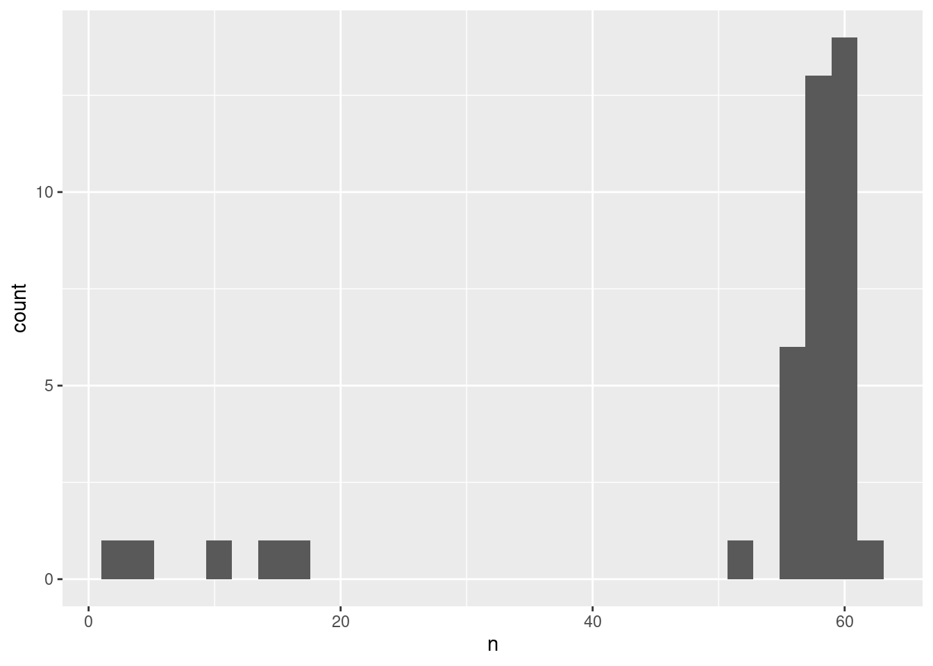
From this initial analysis, we can now proceed to investigate the quantity of beeps sent in more detail. We can proceed to graphically represent the distribution of sent beeps, breaking it down per participant, per dyad, or other relevant levels of analysis. This will allow us to identify any potential discrepancies in the number of beeps sent to each participant/dyad.

This information can be displayed through:

• Histogram plot
• Bar plot: number of beeps sent per id (i.e., participant number).
• Ordered bar plot: similar to the bar plot, but with participants ordered by the number of beeps sent.

data %>% 
  filter(!is.na(sent)) %>% # Keep only sent beeps
  group_by(id) %>% 
  summarize(n = n()) %>% # Compute the number of beeps sent per participant
  ggplot(aes(x=factor(id),y=n)) +
      geom_col(position = "dodge")

data %>% 
  filter(!is.na(sent)) %>% # Keep only sent beeps
  group_by(id) %>% 
  summarize(n = n()) %>% # Compute the number of beeps sent per participant
  mutate(id = factor(id, levels = id[order(n)])) %>% # Order the participants by the number of beeps sent
  ggplot(aes(x=id,y=n)) +
      geom_col(position = "dodge")

data %>% 
  filter(!is.na(sent)) %>% # Keep only sent beeps
  group_by(id) %>% 
  summarize(n = n()) %>% # Compute the number of beeps sent per participant
  ggplot(aes(x=n)) +
    geom_histogram()

Those visualizations will allow us to easily discern patterns or anomalies in beep distribution among individuals. It’s clear that there is a variance in the number of beeps sent to different participants/dyads, which is anormal regarding the study design. This disparity would need to be further investigated to determine if it is due to a technical issue or if it is a result of the study design. Implications for the study at hand must be considered.

Time variables

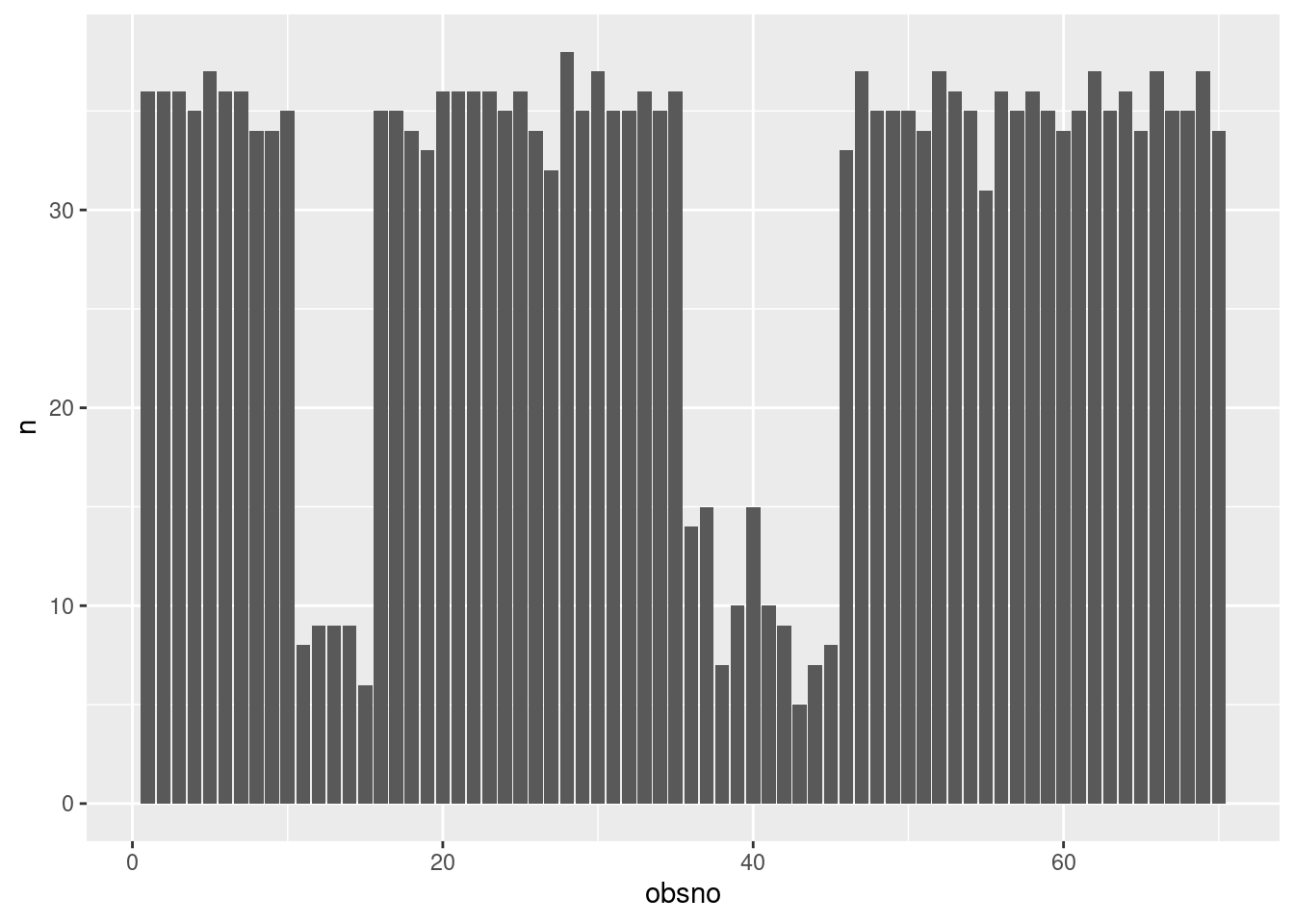
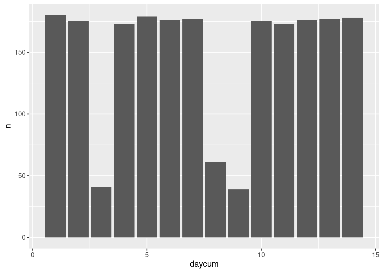
Another good practice is to look at the quantity of beeps sent over time. In our study design, the same number of beeps should be sent to each participant on each day and at each observation number. Hence, we can check that the beeps were sent consistently over time. To investigate this, we can create visualizations depicting the number of beeps sent for each observation number (‘obsno’) or day in the study (‘daycum’; see Create time variables topic). Such graphical representations will help us to identify any temporal variations or irregularities in beep distribution.

data %>% filter(!is.na(sent)) %>% 
  group_by(obsno) %>% summarize(n = n()) %>%
  ggplot(aes(x=obsno,y=n)) +
      geom_col(position = "dodge")

data %>% filter(!is.na(sent)) %>% 
  group_by(daycum) %>% summarize(n = n()) %>%
  ggplot(aes(x=daycum,y=n)) +
      geom_col(position = "dodge")

From the above plots, we can see that the number of beeps sent is relatively inconsistent over time. In particular, there are some days with a very low number of beeps sent.

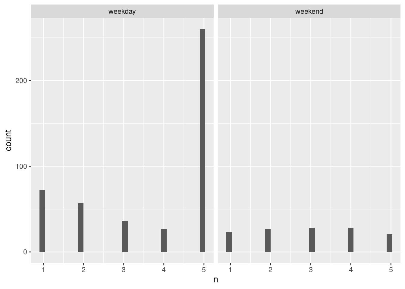
Going a step further, we can integrate 2+ time variables to investigate their potential interaction in their effect on the number of beeps sent. A specific example would be examining the number of beeps sent on a daily basis, segmented by the type of day (weekdays vs. weekends).

data %>% filter(!is.na(sent)) %>% 
  # Compute the type of day
  mutate(wday = ifelse(wday(start) %in% c(1,7), "weekend", "weekday")) %>% 
  # Compute the number of beeps sent per day
  group_by(id, wday, daycum) %>% 
  summarize(n = n()) %>%
  ggplot(aes(x = n)) +
      geom_histogram() +
      facet_wrap(wday~.)

From the above plot, we can see that the number of beeps sent per day (x-axis) is inconsistent across types of days (weekdays vs. weekends). We expected that only days with 5 beeps sent would be present, but we can see that there are a lot of days with fewer beeps sent (i.e., 1, 2, 3, 4). Again, further investigation are required.

Further considerations

Investigating the quantity of sent beeps takes a similar approach to looking at the response rate. Therefore, we can incorporate methodologies (e.g., plots, covariates investigation) from the Response rate topic to further explore the quantity of beeps sent aspect.