Dyadic delay in sending

Packages: dplyr, ggplot2

The sending of the beeps to the participants is often done by an application and/or a server, which can be subject to issues. In the context of ESM dyad studies, it is often expected that the sending of the beeps to the two dyad members should be done at the same time or relatively close in time. It is something we can check.

A important requirement is to reformat your dataframe in a dyad format. In this manipulation, observations from the two dyad members are matched by their observation number and dyad number. A suffix is added to the variable names to differentiate the two dyad members’ observations. For instance, ‘sent_1’ for the sending time variable of partner 1 and ‘sent_2’ for partner 2.

Warning

Errors below can come from wrong data manipulation when creating the ‘data_dyad’ dataframe. Indeed, if the dyad members’ observations are not correctly matched or if observation numbers are not consistent between dyad members, the delay will be computed between two different observations. Hence, it’s advisable to review your code for any potential mistakes when merging the dyad members’ observations.

After reformating, we compute the absolute delay between the dyad’s observations for the same observation number and visualize its distribution. Common errors are extreme positive values, indicating extended time lags before the first (or second) partner received the beeps.

# Compute absolute delay in mins
data_dyad = data_dyad %>%
    mutate(dif_sent = abs(as.numeric(difftime(sent_2, sent_1, units="mins")))) 

# Visualize delay
data_dyad %>% 
    ggplot(aes(x = dif_sent)) +
        geom_histogram()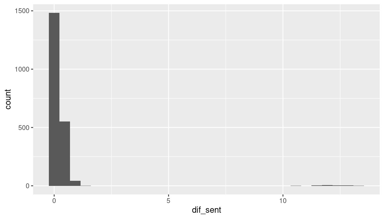

Above, we can see that most of the delays are rather small, with most of the beeps being received by dyad members within 1 minute of each other. However, few beeps were received by dyad members with significant delays (>10 minutes). We can further check those outliers by selecting the rows with a delay greater than 10 minutes:

data_dyad[data_dyad$dif_sent > 10, c("dyad","obsno", "sent_1", "sent_2", "dif_sent")]

     dyad obsno              sent_1              sent_2 dif_sent
35      1    35 2003-03-05 20:36:59 2003-03-05 20:47:24 10.41880
91      2    21 2003-03-03 08:05:39 2003-03-03 08:16:33 10.91043
118     2    48 2003-03-08 14:26:57 2003-03-08 14:15:54 11.05000
221     4    11 2003-03-01 08:28:38 2003-03-01 08:16:24 12.23550
376     6    26 2003-03-04 08:23:34 2003-03-04 08:34:47 11.20789
377     6    27 2003-03-04 11:05:53 2003-03-04 11:16:07 10.23250
387     6    37 2003-03-06 11:30:04 2003-03-06 11:17:52 12.20000
603     9    43 2003-03-07 14:37:03 2003-03-07 14:48:56 11.89411
657    10    27 2003-03-04 11:32:15 2003-03-04 11:19:16 12.97115
675    10    45 2003-03-07 20:18:25 2003-03-07 20:06:27 11.95781
720    11    20 2003-03-02 20:13:54 2003-03-02 20:25:52 11.95872
815    12    45 2003-03-07 20:14:39 2003-03-07 20:26:11 11.53333
1007   15    27 2003-03-04 12:13:39 2003-03-04 12:26:22 12.71895
1155   17    35 2003-03-05 20:31:38 2003-03-05 20:44:13 12.57556
1297   19    37 2003-03-06 11:07:44 2003-03-06 11:20:02 12.30139
1880   27    60 2003-03-10 20:19:17 2003-03-10 20:07:41 11.60733
1896   28     6 2003-02-28 08:23:54 2003-02-28 08:36:28 12.56667
1992   29    32 2003-03-05 11:27:04 2003-03-05 11:15:25 11.65208

Investigating the delay between the dyad members’ observations takes a similar approach to looking at the delay between two consecutive beeps. Therefore, we can incorporate methodologies (e.g., plots, covariates investigation) from the Delay two sent beeps topic to further explore the quantity of beeps sent aspect.