Data characteristics report
The data characteristics report provides a comprehensive summary of the preprocessed data. It encompasses various descriptive analyses which enhances the understanding of the preprocessed data and improves data sharing. Importantly, this report acts as a quality control for the preprocessing workflow. It serves as an additional check to ensure that no errors have been introduced or overlooked during the data manipulation process.
After importing packages and data (including meta-data on the imported packages and data), the report uses the following stucture:
- Section 1: Overview tables. Inclide a codebook table and a participant book.
- Section 2: Study and data characteristics. It encompasses elements from step 1 to 3 of the ESM preprocessing framework.
- Section 3: Variables and processes descriptions. It gives insight into the variables themselves (e.g., distribution, correlation plots, time series).
The esmtools package offers one data characteristics report template for Rmarkdown: ‘data_characteristics_report’ (click to download). An example of a data characteristics report can be found in the repository of the website or at the top of this page. Additionally, a set of specialized functions has been developed that can be useful for this report. Each of these tools is thoroughly described in the Reporting tools section.
The template can be imported into a directory using the ‘use_template()’ function.
esmtools::use_template("data_characteristics_report", output_dir = getwd())More information can be found in the package’s documentation website.
Import packages and data
This section imports the necessary packages and datasets. Specifically for the dataset, we propose two options:
- If you work in synergy with a preprocessing report template, this file can be automatically knitted at the end of the preprocess report. The path to the preprocessed dataset is shared with this data characteristics report through the ‘params’ variable in the header of the document.
- Alternatively, you can specify the path to your preprocessed data, that will be used if no params variable is found.
Additionaly, meta-information can be displayed to enhance transparency, reproducibility and tracability of the elemeents. See the section session and data info.
Section 1. Codebook table
To facilitate data understanding, the report includes a Codebook table. It offers statistics, labels, codes, item wordings, etc. for the variables of interest. You can use the ‘codebook_table()’ function from the esmtools package. Alternatively, an in-depth description of each variable can be included in the ‘Variables and processes descriptions part’ (see Codebook packages section)
Section 2. Study and data characteristics
This section provides elements that correspond to the 4 first steps of the ESM preprocessing framework:
- valuable information about the general characteristics of the dataset (e.g., duplicated observations, distribution of missing values).
- a comprehensive overview of key aspects related to the adherence of data to the predefined sampling scheme and study design.
- participants’ compliance with non-problematic response behaviors.
Interestingly, you can reuse part of your R code from the preprocessing report, with the key distinction being that this code is now executed on the final preprocessed data instead of the data that is undergoing preprocessing. Hence, the plots should be now exempt from errors, previously solved during preprocessing steps.
Section 3. Variables and processes descriptions
In this section, a selection of relevant plots is displayed that help to investigate variables’ interdependence, the within and between differences (e.g., in time series, variable distributions), and patterns in the variables (e.g., variation of response in function of a time variable). Step 5 topics are particularly relevant for this section.
For instance, it can be interesting to investigate the correlation structure between the variables.
To this end, the function ‘ggpairs()’ from the GGally package is particularly relevant.
library(GGally)
var_names = c("PA1","PA2","PA3","NA1","NA2","NA3")
data_mat = na.omit(data[,var_names])
ggpairs(data_mat)
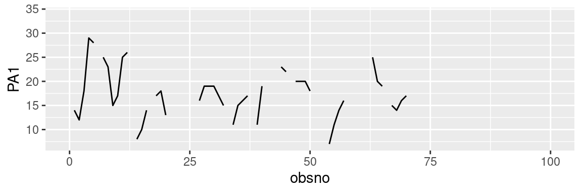
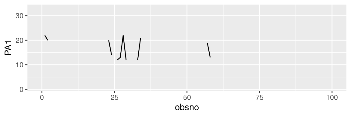
Additionally, one can be interested in displaying same plot for each participant or dyad, such as time series for a variable of interest. To this end we propose different methods:
- ‘facet_wrap()’: This method involves creating multiple small plots arranged in a grid, where each plot represents a distinct subset of the data defined by a categorical variable (e.g., ‘id’). The layout and appearance of the plot can be further customized using the ‘ncols’ (or ‘nrows’) argument, which specifies the desired number of columns for the grid arrangement. Additionally, adjusting the size of the displayed plot can be achieved by utilizing the ‘fig.width’ and ‘fig.height’ options within the R code chunk. An alternative to this function is the ‘facet_grid()’ function.
- repetition of plots: create identical plots for each participant within a loop. This is accomplished by defining two functions: one for the plot itself (e.g., ‘plot_1()’), and another function (‘display_plots()’) that creates the plot for each subgroup in the dataframe. The size of the displayed plots can be adjusted using the ‘fig.width’ and ‘fig.height’ options. It is important to note that the R code chunk containing this method should have the option “results=‘asis’” in order to display the plots as intended.
# Reduce the number of participant for demonstration purpuse
df = data[data$id < 10,]

ggplot(data = df, aes(x = obsno, y = PA1)) +
  geom_line() +
  facet_wrap(id~., ncol=3) +
  scale_x_continuous(limits=c(0,100))
Participant book
In a sub-section, you can include a Participant book. It captures participants’ response behaviors (e.g., compliance, study duration, start time) alongside with descriptive statistics and time series plots for the variables of interest and each participant.


