Item response time
Packages: dplyr, tidyr, ggplot2
Rather than investigating the time needed to answer a whole observation, we can investigate it for each item, which provides an in-depth exploration of the participants’ response behaviors. Nonetheless, it requires that the items are displayed one after the other (or at least by groups of items) on the screen and that the timestamps of every validation to each item (group of items) are recorded. In addition, it requires general preprocessing, such as the presence of missing values (see step 1), in addition to a more specific one if the items were randomly displayed to the participants.
Note that the time per item can also be computed by dividing the time needed to answer the whole observation by the number of items (whenever the times to fulfill items are not recorded individually). Nonetheless, it won’t add more information than looking at the time to answer a beep, except if the number of items displayed at each beep is inconsistent.
Know the timestamps order and compute scores
To compute the time per item and its standard deviation, we first need to know whether the items were presented in a random order to the participant or not. Below we show the two versions of the same dataset:
- Not randomly displayed: items were displayed in the same order as the variables in the dataframe for each participant.
- Randomly displayed: if the items were presented in a random order, then we will need to reorder them for each observation independently. In our example, the order was recorded in another variable ‘order_vars’. It takes the form of a string such as: “NA3,PA3,PA1,PA2,NA2,NA1,…” in ;the ‘data_time_rand’ dataset.
head(na.omit(data_time)) dyad id obsno sent start end
4 1 1 4 2018-10-17 12:59:52 2018-10-17 13:00:12 2018-10-17 13:03:01
7 1 1 7 2018-10-18 10:59:53 2018-10-18 11:00:02 2018-10-18 11:01:57
8 1 1 8 2018-10-18 12:00:27 2018-10-18 12:00:41 2018-10-18 12:02:22
9 1 1 9 2018-10-18 13:00:13 2018-10-18 13:00:30 2018-10-18 13:03:40
12 1 1 12 2018-10-19 11:00:17 2018-10-19 11:00:38 2018-10-19 11:01:30
13 1 1 13 2018-10-19 12:00:15 2018-10-19 12:00:54 2018-10-19 12:00:58
PA1_time PA2_time PA3_time
4 2018-10-17 13:00:37 2018-10-17 13:01:03 2018-10-17 13:01:25
7 2018-10-18 11:00:22 2018-10-18 11:00:37 2018-10-18 11:00:48
8 2018-10-18 12:00:54 2018-10-18 12:01:09 2018-10-18 12:01:22
9 2018-10-18 13:01:02 2018-10-18 13:01:24 2018-10-18 13:01:45
12 2018-10-19 11:00:52 2018-10-19 11:00:53 2018-10-19 11:00:55
13 2018-10-19 12:00:54 2018-10-19 12:00:54 2018-10-19 12:00:55
NA1_time NA2_time NA3_time
4 2018-10-17 13:01:53 2018-10-17 13:02:07 2018-10-17 13:02:36
7 2018-10-18 11:00:57 2018-10-18 11:01:19 2018-10-18 11:01:31
8 2018-10-18 12:01:39 2018-10-18 12:01:55 2018-10-18 12:02:12
9 2018-10-18 13:02:21 2018-10-18 13:02:47 2018-10-18 13:03:07
12 2018-10-19 11:01:03 2018-10-19 11:01:19 2018-10-19 11:01:21
13 2018-10-19 12:00:59 2018-10-19 12:01:01 2018-10-19 12:01:02
contact_time location_time
4 2018-10-17 13:02:55 2018-10-17 13:03:01
7 2018-10-18 11:01:54 2018-10-18 11:01:57
8 2018-10-18 12:02:19 2018-10-18 12:02:22
9 2018-10-18 13:03:36 2018-10-18 13:03:40
12 2018-10-19 11:01:34 2018-10-19 11:01:30
13 2018-10-19 12:01:05 2018-10-19 12:00:58Hence, we propose 2 methods to compute the time per item (in seconds). In particular, the method for the random condition needs to take into account the order the observations were displayed every time. Note that the ‘start’ variable and/or the ‘end’ variable are also both needed.
In the provided examples, the timestamp associated with each variable corresponds to the time at which the participant ended the item. If, in your collected data, the timestamps are associated with the time at which the participant initiated the item, you need to make adjustments to the following code.
You must make sure that the timestamp variables are in a time format (e.g. POSIXct).
# Select subset of variables
df_raw_time = data_time %>% dplyr::select(start, PA1_time:location_time)

# Prepare a NA dataframe to store the computed values
df_time = data.frame(matrix(NA, nrow = nrow(df_raw_time), ncol = ncol(df_raw_time)-1))
names(df_time) = names(df_raw_time)[2:ncol(df_raw_time)]

# Loop over each timestamp column: compute the difference in seconds between col and col+1
for (col in 1:(ncol(df_raw_time)-1)){
  time_dif = difftime(df_raw_time[,col+1], df_raw_time[,col], units="sec")
  df_time[,col] = time_dif
}

# Add dyad, id, obsno columns
df_time = cbind(data_time[,c("dyad","id","obsno")], df_time)
# Reformat to numerical values
df_time = df_time %>% mutate(across(PA1_time:location_time, as.numeric))Finally, based on the time per item scores, we can compute, for each observation, the standard deviation of the time per item over the different items.
subset = df_time %>% select(PA1_time:location_time)
df_time$sd_time = apply(subset, 1, sd, na.rm=TRUE)
Check coherence of timestamps
Before going further, looking at unexpected values of the time per item is a good way to check the coherence between the timestamp variables (e.g. order of the item not been consistent with the timestamp order). In particular, we can look for negative values, which would represent later planned items with an earlier timestamp than the previous item.
We can compute the number of times the condition is met for each row. If the condition is met at least one time in a row, then it would indicate a potential issue.
subset = df_time %>% select(PA1_time:location_time)
thres_low = 0
thres_high = 1800
df_time$time_test = apply(subset, 1, function(x){ sum(x <= thres_low | x >= thres_high)})
We can first compute the number of occurence:
sum(df_time$time_test > 0, na.rm=TRUE)[1] 1685We can observe here that it occurred more than once. In such a case, it is crucial to initiate an investigation into these specific rows and attempt to identify the root(s) cause of the issue and try to find a solution to solve it (them).
Investigations
After the previous preprocessing steps, we can have an in-depth exploration of the participants’ response behaviors using the two computed metrics: time per item and the standard deviation of the time per item (within observations).
Time per item
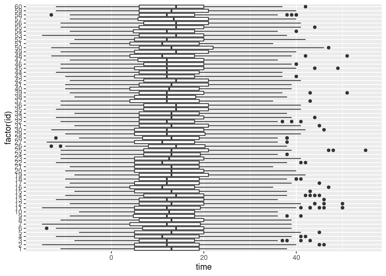
Specifically for the time per item, we can plot their distributions following different conditions:
Standard deviation
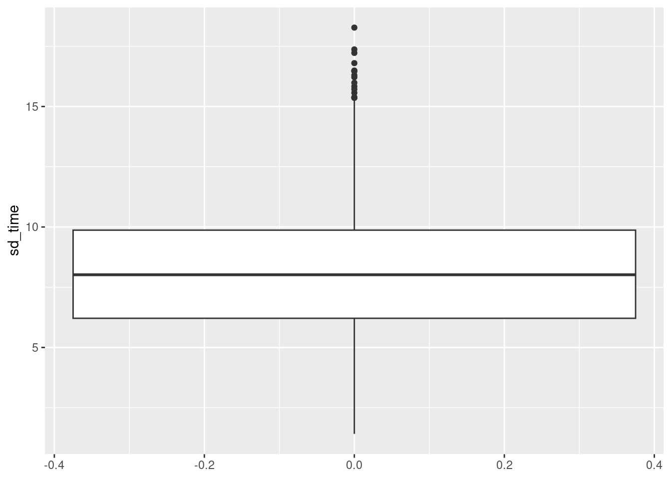
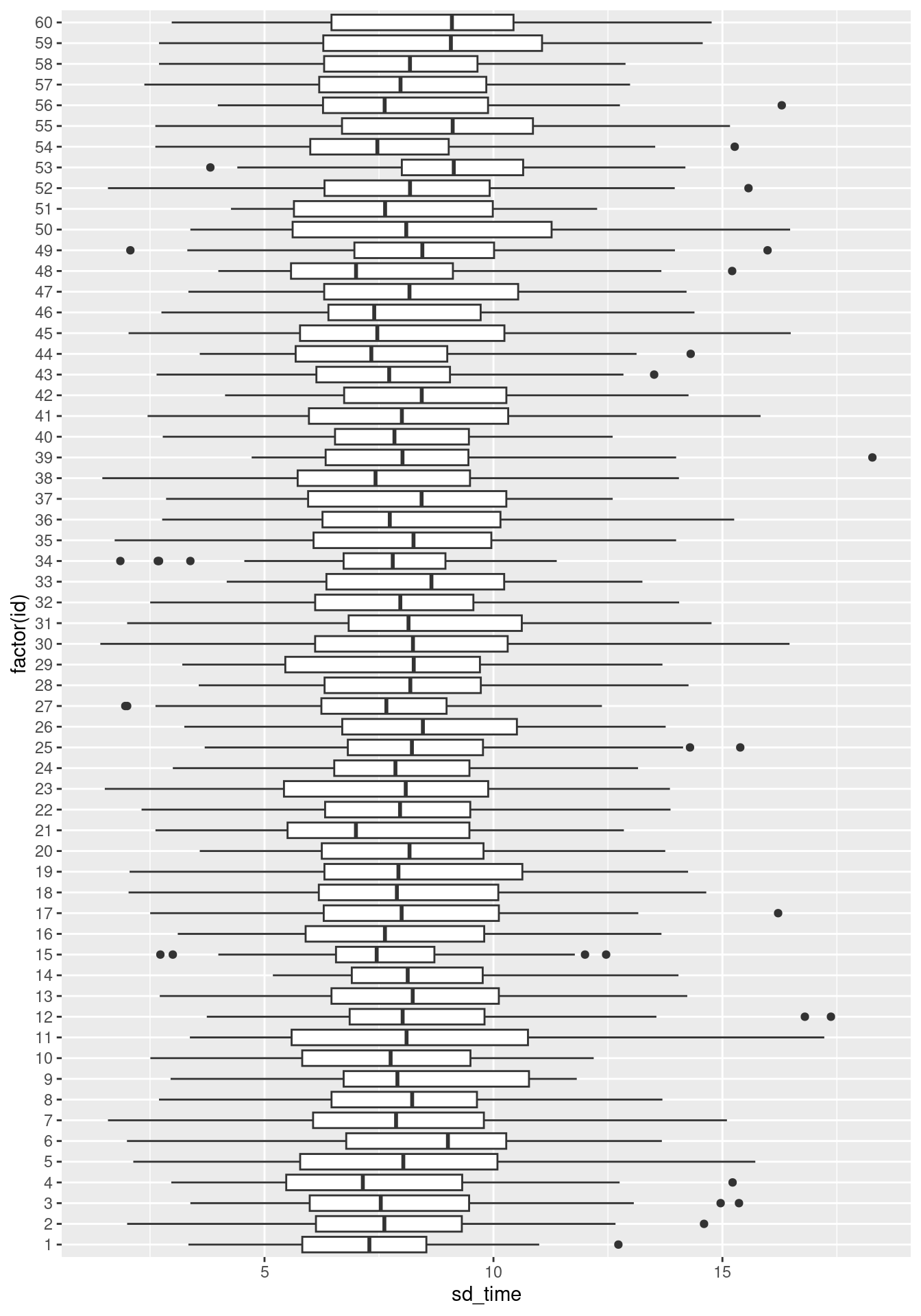
For the standard deviation of the time per item, we can also investigate their distributions in multiple ways:


